Cassandra Query Language (CQL)
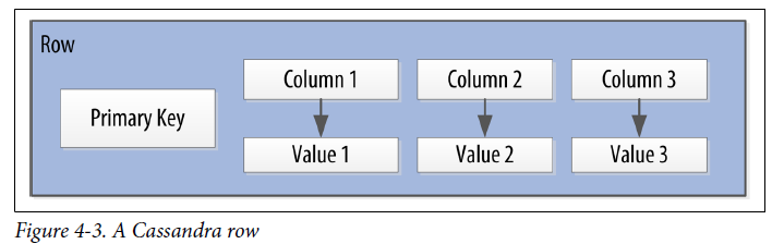
Cassandra can be classified as a wide column store.
Cassandra uses a special type of primary key called a composite key (or compound key) to represent groups of related rows, also called partitions.
The composite key consists of a partition key, plus an optional set of clustering columns.
The partition key is used to determine the nodes on which rows are stored and can itself consist of multiple columns.
The clustering columns are used to control how data is sorted for storage within a partition. Cassandra also supports an additional construct called a static column, which is for storing data that is not part of the primary key but is shared by every row in a partition.

Cassandra Data Model: Partitions
A partitioner determines how data is distributed across the nodes in the cluster. Cassandra organizes rows in partitions. Each row has a partition key that is used to identify the partition to which it belongs. A partitioner, then, is a hash function for computing the token of a partition key. Each row of data is distributed within the ring according to the value of the partition key token.
The role of the partitioner is to compute the token based on the partition key columns. Any clustering columns that may be present in the primary key are used to determine the ordering of rows within a given node that owns the token representing that partition.

Cassandra provides several different partitioners:
Murmur3Partitioner
RandomPartitioner
Distributed Architecture: Ring And Tokens
Cassandra represents the data managed by a cluster as a ring. Each node in the ring is assigned one or more ranges of data described by a token, which determines its position in the ring.
For example: In the default configuration, a token is a 64-bit integer ID used to identify each partition. This gives a possible range for tokens
from −2^63 to 2^63−1.
A node claims ownership of the range of values less than or equal to each token and
greater than the last token of the previous node, known as a token range.
The node with the lowest token owns the range less than or equal to its token and the
range greater than the highest token, which is also known as the wrapping range.
In this way, the tokens specify a complete ring.

Data is assigned to nodes by using a hash function to calculate a token for the
partition key. This partition key token is compared to the token values
for the various nodes to identify the range, and therefore the node that owns the data.
cqlsh:my_keyspace> SELECT last_name, first_name, token(last_name) FROM user;
last_name | first_name | system.token(last_name)
-----------+------------+-------------------------
Rodriguez | Mary | -7199267019458681669
Scott | Isaiah | 1807799317863611380
Nguyen | Bill | 6000710198366804598
Nguyen | Wanda | 6000710198366804598
(5 rows)
Distributed Architecture: Vnodes
Instead of assigning a single token to a node, the token range is broken up into multiple smaller ranges. Each physical node is then assigned multiple tokens. Historically, each node has been assigned 256 of these tokens, meaning that it represents 256 virtual nodes.
Vnodes make it easier to maintain a cluster containing heterogeneous machines. For nodes in your cluster that have more computing resources available to them, you can increase the number of vnodes by setting the num_tokens property in the cassandra.yaml file.
Cassandra automatically handles the calculation of token ranges for each node in the cluster in proportion to their num_tokens value.
Vnodes make it easier to maintain a cluster containing heterogeneous machines. For nodes in your cluster that have more computing resources available to them, you can increase the number of vnodes by setting the num_tokens property in the cassandra.yaml file.
Distributed Architecture: Gossip
To support decentralization and partition tolerance, Cassandra uses a gossip protocol that allows each node to keep track of state information about the other nodes in the cluster. The gossiper runs every second on a timer.
When the gossiper determines that another endpoint is dead, it "convicts” that endpoint by marking it as dead in its local list and logging that fact.
Distributed Architecture: Snitch
Snitch is to provide information about your network topology so that Cassandra can efficiently route requests.
The snitch will figure out where nodes are in relation to other nodes.
The snitch will determine relative host proximity for each node in a cluster, which is used to determine which nodes to read and write from.
For example we’ll see how snitch participates in read operation: When
Cassandra performs a read, it must contact a number of replicas determined by the consistency level.
In order to support the maximum speed for reads, Cassandra selects a single replica to query for the full object, and asks additional replicas for hash values in order to ensure the latest version of the requested data is returned. The snitch helps to help identify the replica that will return the fastest, and this is the replica which is queried for the full data.
SimpleSnitch(Default): It is topology unaware; that is, it does not know
about the racks and data centers in a cluster, which makes it unsuitable for multiple data center deployments.
While Cassandra provides a pluggable way to statically describe your cluster’s topology, it also provides a feature called dynamic snitching that helps optimize the routing of reads and writes over time.Your selected snitch is wrapped with another snitch called the
DynamicEndpointSnitch. The dynamic snitch gets its basic understanding of the topology from the selected snitch. It then monitors the performance of requests to the other nodes, even keeping track of things like which nodes are performing compaction.
The performance data is used to select the best replica for each query. This enables Cassandra to avoid routing requests to replicas that are busy or performing poorly.
Replication/Consistency: Replication
A node serves as a replica for different ranges of data. If one node
goes down, other replicas can respond to queries for that range of
data. Cassandra replicates data across nodes in a manner
transparent to the user, and the replication factor is the number of
nodes in your cluster that will receive copies (replicas)
of the same data. If your replication factor is 3, then three nodes in
the ring will have copies of each row.
The first replica will always be the node that claims the range in
which the token falls, but the remainder of the replicas are placed
according to the replication strategy (replica placement strategy).
Out of the box, Cassandra provides two primary implementations of
this interface (AbstractReplicationStrategy)
SimpleStrategy: places replicas at consecutive nodes around the ring,
starting with the node indicated by the partitioner
NetworkTopologyStrategy: This allows you to specify a different
replication factor for each data center. Within a data center, it allocates
replicas to different racks in order to maximize availability.
Recommended for keyspaces in production deployments.
Replication/Consistency: Consistency
Cassandra provides tunable consistency levels that allow you to
make these trade-offs at a fine-grained level.
You specify a consistency level on each read or write query that
indicates how much consistency you require. A higher consistency
level means that more nodes need to respond to a read or write query,
giving you more assurance that the values present on each replica are
the same.
For read queries, the consistency level specifies how many replica
nodes must respond to a read request before returning the data.
For write operations, the consistency level specifies how many replica
nodes must respond for the write to be reported as successful to the
client. Because Cassandra is eventually consistent, updates to other
replica nodes may continue in the background.
The available consistency levels include ONE, TWO, and THREE,
each of which specify an absolute number of replica nodes that must
respond to a request. The QUORUM consistency level requires a
response from a majority of the replica nodes.
Expressed as:
Q = floor (RF/2 + 1)
Q - the number of nodes needed to achieve quorum for a replication
factor RF.
The ALL consistency level requires a response from all of the replicas.
Consistency is tuneable in Cassandra because clients can specify the
desired consistency level on both reads and writes.
Recommended way to achieve strong consistency in Cassandra
is to write and read using the QUORUM or LOCAL_QUORUM
consistency levels.
Distinguishing Consistency Levels and Replication Factors
If you’re new to Cassandra, it can be easy to confuse the concepts
of replication factor and consistency level.
The replication factor is set per keyspace. The consistency level
is specified per query, by the client. The replication factor indicates
how many nodes you want to use to store a value during each write
operation. The consistency level specifies how many nodes the client
has decided must respond in order to feel confident of a successful
read or write operation. The confusion arises because the consistency
level is based on the replication factor, not on the number of nodes in
the system.
Queries and Coordinator Nodes
Let’s bring these concepts together to discuss how Cassandra nodes
interact to support reads and writes from client applications.

A client may connect to any node in the cluster to initiate a read or
write query. This node is known as the coordinator node. The
coordinator identifies which nodes are replicas for the data that is
being written or read and forwards the queries to them.
For a write, the coordinator node contacts all replicas, as determined
by the consistency level and replication factor, and considers the write
successful when a number of replicas commensurate with the
consistency level acknowledge the write.
For a read, the coordinator contacts enough replicas to ensure the
required consistency level is met, and returns the data to the client.
Replication/Consistency: Hinted Handoff (HA Mechanism)
When a write request is sent to cassandra but a replica node is not
available because of failure then the coordinator node would create a
post it note that contains the information from the write request. Once
the node is back online, it is detected through the gossip and hint is
handed off to the node.
Cassandra holds a separate hint for each partition that is to be written.
Hinted handoff is used in Amazon’s Dynamo, which inspired the design of
databases, including Cassandra and Amazon’s DynamoDB.
It is also familiar to those who are aware of the concept of guaranteed
delivery in messaging systems such as the Java Message Service
(JMS). In a durable guaranteed-delivery JMS queue, if a message
cannot be delivered to a receiver, JMS will wait for a given interval
and then resend the request until the message is received.
If the node is offline for some time the hints get piled up and once the
node is back online the hints flood the node. To avoid this situation
Cassandra limits the storage of hints to a configurable time window.
It is also possible to disable hinted handoff entirely.
Because of the limitation mentioned above maintaining consistency
of the data becomes difficult.
For achieving the consistency in cassandra anti-entropy protocol is
used.
Anti-entropy protocols are a type of gossip protocol for repairing the
replicated data. They work by comparing the replicas and reconcile
the differences observed among them.
Anti-entropy is used in Amazon DynamoDB.
In cassandra Replica synchronization is supported via two different
modes:
Read repair: Read repair refers to the synchronization of replicas as
data is read.
Anti-entropy repair: Is a manually initiated operation performed on
nodes as part of a regular maintenance process. Done using nodetool.
Both Cassandra and Dynamo use Merkle trees for anti-entropy, but
their implementations are a little different. In Cassandra, each table
has its own Merkle tree; the tree is created as a snapshot during a
validation compaction, and is kept only as long as is required to send
it to the neighboring nodes on the ring. The advantage of this
implementation is that it reduces network I/O.
Lightweight Transactions and Paxos
Strong consistency is not enough to prevent race conditions in cases
where clients need to read, then write data.
A scenario to explain:
In creating a new user account, we’d like to make sure that the user
record doesn’t already exist, lest we unintentionally overwrite existing
user data. So first we do a read to see if the record exists, and then
only perform the create if the record doesn’t exist.
The behavior we’re looking for is called linearizable consistency,
meaning that we’d like to guarantee that no other client can come in
between our read and write queries with their own modification.
Cassandra supports a lightweight transaction (LWT) mechanism that
provides linearizable consistency.
Cassandra’s LWT implementation is based on Paxos. Paxos is a
consensus algorithm that allows distributed peer nodes to agree on a
proposal, without requiring a leader to coordinate a transaction.
Paxos and other consensus algorithms emerged as alternatives to
traditional two-phase commit-based approaches to distributed
transactions.
Paxos algorithm have two stages:
Prepare/promise
Propose/accept.
To modify data, a coordinator node can propose a new value to the
replica nodes, taking on the role of leader. Other nodes may act as
leaders simultaneously for other modifications.
Each replica node checks the proposal, and if the proposal is the
latest it has seen, it promises to not accept proposals associated with
any prior proposals.
Each replica node also returns the last proposal it received that is still
in progress.
If the proposal is approved by a majority of replicas, the leader
commits the proposal, but with the caveat that it must first commit any
in-progress proposals that preceded its own proposal.
The Cassandra implementation extends the basic Paxos algorithm to
support the desired read-before-write semantics (also known as
check-and-set), and to allow the state to be reset between
transactions. It does this by inserting two additional phases into the
algorithm, so that it works as follows:
1. Prepare/Promise
2. Read/Results
3. Propose/Accept
4. Commit/Ack
Thus, a successful transaction requires four round-trips between the
coordinator node and replicas. This is more expensive than a regular
write, which is why you should think carefully about your use case
before using LWTs.
Cassandra’s lightweight transactions are limited to a single partition.
Internally, Cassandra stores a Paxos state for each partition.
This ensures that transactions on different partitions cannot interfere
with each other.
Memtables, SSTables, and Commit Logs
When a node receives a write operation, it immediately writes the
data to a commit log. The commit log is a crash-recovery mechanism
that supports Cassandra’s durability goals. A write will not count as
successful on the node until it’s written to the commit log, to ensure
that if a write operation does not make it to the in-memory store
(memtable), it will still be possible to recover the data. If you shut down
the node or it crashes unexpectedly, the commit log can ensure that
data is not lost. That’s because the next time you start the node,
the commit log gets replayed. In fact, that’s the only time the commit
log is read; clients never read from it.
CREATE KEYSPACE my_keyspace WITH replication =
{'class': 'SimpleStrategy', 'replication_factor': '1'} AND durable_writes =true;
The durable_writes property controls whether Cassandra will use the
commit log for writes to the tables in the keyspace. This value defaults
to true, meaning that the commit log will be updated on modifications.
Setting the value to false increases the speed of writes, but also risks
losing data if the node goes down before the data is flushed from
memtables into SSTables.
After it’s written to the commit log, the value is written to a
memory-resident data structure called the memtable. Each memtable
contains data for a specific table.
Prior to 2.1 version memtables were in JVM. Now a configuration
option is available to specify the amount of on-heap and native
memory.
When the number of objects stored in the memtable reaches a
threshold, the contents of the memtable are flushed to disk in a file
called an SSTable (Sorted String Table). Multiple memtables are
created for a single table. One current and other one waiting to be
flushed.
Each commit log maintains an internal bit flag to indicate whether it
needs flushing. When a write operation is first received, it is written to
the commit log and its bit flag is set to 1.
Once a memtable is flushed to disk as an SSTable, it is immutable and
cannot be changed by the application. Despite the fact that SSTables
are compacted, this compaction changes only their on-disk
representation; it essentially performs the “merge” step of a mergesort
into new files and removes the old files on success.
All writes are sequential, which is the primary reason that writes
perform so well in Cassandra. No reads or seeks of any kind are
required for writing a value to Cassandra because all writes are
append operations. This makes the speed of your disk one key
limitation on performance.
On reads, Cassandra will read both SSTables and memtables to find
data values, as the memtable may contain values that have not yet
been flushed to disk.
Bloom Filters
Bloom filters are used to boost the performance of reads.
Bloom filters work by mapping the values in a data set into a bit array
and condensing a larger data set into a digest string using a hash
function. The digest, by definition, uses a much smaller amount of
memory than the original data would. The filters are stored in memory
and are used to improve performance by reducing the need for disk
access on key lookups. Disk access is typically much slower than
memory access. So, in a way, a Bloom filter is a special kind of key
cache.
Cassandra maintains a Bloom filter for each SSTable. When a query is
performed, the Bloom filter is checked first before accessing the disk.
Caching
Mechanism to boost read performance, three optional forms of caching:
• The key cache stores a map of partition keys to row index entries,
facilitating faster read access into SSTables stored on disk. The key cache is stored on the JVM heap.
• The row cache caches entire rows and can greatly speed up read
access for frequently accessed rows, at the cost of more memory
usage. The row cache is stored in off-heap memory.
• The counter cache was added in the 2.1 release to improve counter
performance by reducing lock contention for the most frequently
accessed counters.
By default, key and counter caching are enabled, while row caching is
disabled, as it requires more memory.
Compaction
SSTables are immutable, which helps Cassandra achieve such high write speeds.
Periodic compaction of these SSTables is important in order to support
fast read performance and clean out stale data values.
A compaction operation in Cassandra is performed in order to merge SSTables.
During compaction, the data in SSTables is merged: the keys are
merged, columns are combined, obsolete values are discarded, and a new index is created.
Compaction is the process of freeing up space by merging large
accumulated datafiles. This is roughly analogous to rebuilding a table
in the relational world.
On compaction, the merged data is sorted, a new index is created
over the sorted data, and the freshly merged, sorted, and indexed data
is written to a single new SSTable (each SSTable consists of multiple
files, including Data, Index, and Filter).
Cassandra supports multiple algorithms for compaction via the strategy
pattern. The compaction strategy is an option that is set for each table.
• SizeTieredCompactionStrategy (STCS) is the default compaction
strategy and is recommended for write-intensive tables
• LeveledCompactionStrategy (LCS) is recommended for read-intensive tables
• TimeWindowCompactionStrategy (TWCS) is intended for time series or otherwise date-based data.
Users with prior experience may recall that Cassandra exposes an
administrative operation called major compaction (also known as full
compaction) that consolidates multiple SSTables into a single SSTable. While this
feature is still available, the utility of performing a major compaction has been greatly reduced over time.
In fact, usage is actually discouraged in production environments, as it tends to limit
Cassandra’s ability to remove stale data.
Deletion and Tombstones
To prevent deleted data from being reintroduced, Cassandra uses a
concept called a tombstone. A tombstone is a marker that is kept to
indicate data that has been deleted. When you execute a delete
operation, the data is not immediately deleted. Instead, it’s treated as
an update operation that places a tombstone on the value.
A tombstone is similar to the idea of a “soft delete” from the relational
world. Instead of actually executing a delete SQL statement, the application will issue an update statement that changes a value in a
column called something like “deleted.” Programmers sometimes do
this to support audit trails. As you might expect, we see a different
token for each partition, and the same token appears for the two rows
represented by the partition key value “Nguyen.”
List all tables in a keyspace
cqlsh>use <keyspace>;
cqlsh:<keyspace>>describe tables;
    (or)
cqlsh:<keyspace>>desc tables;
Export results of cassandra query to CSV file:
First option from Unix prompt
$ bin/cqlsh -e "select * from keyspace.tablename where <condition>" > /root/tablename_results.csv
Second option From CQL Shell
cqlsh> CAPTURE '/root/tablename_results.csv';
cqlsh> select * from keyspace.tablename where <condition>;
cqlsh> CAPTURE OFF
Files generated from the above options would be pipe(|) separated. To replace the pipe with comma(,) using the following command:
$ sed -i -e 's/|/,/g' /root/tablename_results.csv
Creating table:
CREATE TABLE IF NOT EXISTS testkeyspace.testtable (
id timeuuid,
testcol1 int,
testcol2 text,
PRIMARY KEY ((testcol1), id));
WITH CLUSTERING ORDER BY (testcol1 DESC);
Inserting records in a table:
INSERT INTO testkeyspace.testtable (testcol1, testcol2) VALUES (1111, 'testval');
Node tool commands:
nodetool refresh testkeyspace testtable
nodetool repair keyspace testkeyspace tables testtable

Provides usage statistics of thread pools
nodetool tpstats

Provides statistics about one or more tables.
nodetool tablestats
Start/Stop/Status of DSE service:
sudo service dse stop
sudo service dse start
sudo service dse status
Start and stop of data stax agent:
sudo service datastax-agent start
sudo service datastax-agent restart
ps -ef | grep datastax-agent
Data Stax file system (DSEFS)
Get the file from DSEFS to local file system:
Syntax
dse fs "get <dsefs filepath> <localfilepath>"
Example: get test.csv
dse fs "get /myfolder/test.csv /root/test.csv"
Put the file to DSEFS from local file system:
Syntax:
dse fs "put -o <localfilepath> <dsefs path>"

Example:to upload test.csv
dse fs "put -o /root/test.csv /myfolder/test.csv"